Week 3 - Machine Learning
Classification, Representation, Logistic Regression Model, Multiclass Classification

Classification
Now we are switching from regression problems to classification problems. Don’t be confused by the name “Logistic Regression”; it is named that way for historical reasons and is actually an approach to classification problems, not regression problems.
Binary Classification Problem
y can take on only two values, 0 and 1
Hypothesis Representation
We could approach the classification problem ignoring the fact that y is discrete-valued, and use our old linear regression algorithm to try to predict y given x. However, it is easy to construct examples where this method performs very poorly.
Hypothesis should satisfy:
$$0 \leq h_\theta(x) \leq 1$$
Sigmoid Function, also called Logistic Function:
$$ h_\theta (x) = g ( \theta^T x ) \\ z = \theta^T x \\ g(z) = \dfrac{1}{1 + e^{-z}} $$
$h_\theta$ will give us the probability:
$$ h_\theta(x) = P(y=1 | x ; \theta) = 1 - P(y=0 | x ; \theta) \\ P(y = 0 | x;\theta) + P(y = 1 | x ; \theta) = 1 $$
Simplied probability function:
$$ P(y|x) = h_\theta(x)^{y} (1 - h_\theta(x))^{1-y} $$
So in order to decease the cost:
$$ \begin{align} \uparrow \log(P(y|x)) & = \log(h_\theta(x)^{y} (1 - h_\theta(x))^{1-y}) \newline & = y \log(h_\theta(x)) + (1-y) \log(1 - h_\theta(x)) \newline & = - J(\theta) \downarrow \end{align} $$
Decision Boundary
The decision boundary is the line that separates the area where y = 0 and where y = 1.
$$ \begin{align} h_\theta(x) & \geq 0.5 \rightarrow y = 1 \newline h_\theta(x) & < 0.5 \rightarrow y = 0 \newline g(z) & \geq 0.5 \quad when \; z \geq 0 \end{align} $$
So:
$$ \begin{align} \theta^T x < 0 & \Rightarrow y = 0 \newline \theta^T x \geq 0 & \Rightarrow y = 1 \end{align} $$
Cost Function
We cannot use the same cost function that we use for linear regression because the Logistic Function will cause the output to be wavy, causing many local optima. In other words, it will not be a convex function.
Instead, our cost function for logistic regression looks like:
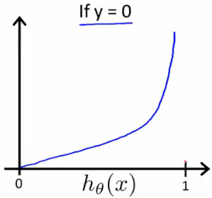
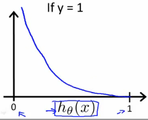
$$ \begin{align} & J(\theta) = \dfrac{1}{m} \sum_{i=1}^m \mathrm{Cost}(h_\theta(x^{(i)}),y^{(i)}) \newline & \mathrm{Cost}(h_\theta(x),y) = -\log(h_\theta(x)) \; & \text{if y = 1} \newline & \mathrm{Cost}(h_\theta(x),y) = -\log(1-h_\theta(x)) \; & \text{if y = 0} \end{align} $$
$J(\theta)$ vs. $h_\theta(x)$:
$$ \begin{align} & \text{ if } h_\theta(x) = y & \mathrm{Cost}(h_\theta(x),y) = 0 \newline & \text{ if } y = 1 \; \mathrm{and} \; h_\theta(x) \rightarrow 0 & \mathrm{Cost}(h_\theta(x),y) \rightarrow \infty \newline & \text{ if } y = 0 \; \mathrm{and} \; h_\theta(x) \rightarrow 1 & \mathrm{Cost}(h_\theta(x),y) \rightarrow \infty \newline \end{align} $$
Simplified Cost Function and Gradient Descent
Compress our cost function’s two conditional cases into one case:
$$\mathrm{Cost}(h_\theta(x),y) = - y \; \log(h_\theta(x)) - (1 - y) \log(1 - h_\theta(x))$$
Entire cost function:
$$ J(\theta) = - \frac{1}{m} \sum_{i=1}^m[y^{(i)} log(h_\theta(x^{(i)})) + (1 - y^{(i)})log(1 - h_\theta(x^{(i)}))] $$
A vectorized implementation is:
$$ \begin{align} & h = g(X\theta)\newline & J(\theta) = \frac{1}{m} \cdot \left(-y^{T}\log(h)-(1-y)^{T}\log(1-h)\right) \end{align} $$
Gradient Descent
This algorithm is identical to the one we used in linear regression. We still have to simultaneously update all values in theta. $$ \begin{align} & Repeat \; \lbrace \newline & \; \theta_j := \theta_j - \frac{\alpha}{m} \sum_{i=1}^m (h_\theta(x^{(i)}) - y^{(i)}) x_j^{(i)} \newline & \rbrace \end{align} $$
In linear regression $h_\theta(x) = \theta^T x$, while in logistic regression $h_\theta(x) = \frac{1}{1 + e^{-\theta^T x}}$
A vectorized implementation is:
$$ \theta := \theta - \frac{\alpha}{m} X^T (g(X\theta) - \vec{y}) $$
Partial derivative of J(θ)
First calculate derivative of sigmoid function:
$$ \begin{align} \sigma(x)’&=\left(\frac{1}{1+e^{-x}}\right)‘=\frac{-(1+e^{-x}) ‘}{(1+e^{-x})^2}=\frac{-1’-(e^{-x})‘}{(1+e^{-x})^2}=\frac{0-(-x)‘(e^{-x})}{(1+e^{-x})^2}=\frac{-(-1)(e^{-x})}{(1+e^{-x})^2}=\frac{e^{-x}}{(1+e^{-x})^2} \newline &=\left(\frac{1}{1+e^{-x}}\right)\left(\frac{e^{-x}}{1+e^{-x}}\right)=\sigma(x)\left(\frac{+1-1 + e^{-x}}{1+e^{-x}}\right)=\sigma(x)\left(\frac{1 + e^{-x}}{1+e^{-x}} - \frac{1}{1+e^{-x}}\right)=\sigma(x)(1 - \sigma(x)) \end{align} $$
Resulting partial derivative:
$$ \begin{align} \frac{\partial}{\partial \theta_j} J(\theta) &= \frac{\partial}{\partial \theta_j} \frac{-1}{m}\sum_{i=1}^m \left [ y^{(i)} log (h_\theta(x^{(i)})) + (1-y^{(i)}) log (1 - h_\theta(x^{(i)})) \right ] \newline &= - \frac{1}{m}\sum_{i=1}^m \left [ y^{(i)} \frac{\partial}{\partial \theta_j} log (h_\theta(x^{(i)})) + (1-y^{(i)}) \frac{\partial}{\partial \theta_j} log (1 - h_\theta(x^{(i)}))\right ] \newline &= - \frac{1}{m}\sum_{i=1}^m \left [ \frac{y^{(i)} \frac{\partial}{\partial \theta_j} h_\theta(x^{(i)})}{h_\theta(x^{(i)})} + \frac{(1-y^{(i)})\frac{\partial}{\partial \theta_j} (1 - h_\theta(x^{(i)}))}{1 - h_\theta(x^{(i)})}\right ] \newline &= - \frac{1}{m}\sum_{i=1}^m \left [ \frac{y^{(i)} \frac{\partial}{\partial \theta_j} \sigma(\theta^T x^{(i)})}{h_\theta(x^{(i)})} + \frac{(1-y^{(i)})\frac{\partial}{\partial \theta_j} (1 - \sigma(\theta^T x^{(i)}))}{1 - h_\theta(x^{(i)})}\right ] \newline &= - \frac{1}{m}\sum_{i=1}^m \left [ \frac{y^{(i)} \sigma(\theta^T x^{(i)}) (1 - \sigma(\theta^T x^{(i)})) \frac{\partial}{\partial \theta_j} \theta^T x^{(i)}}{h_\theta(x^{(i)})} + \frac{- (1-y^{(i)}) \sigma(\theta^T x^{(i)}) (1 - \sigma(\theta^T x^{(i)})) \frac{\partial}{\partial \theta_j} \theta^T x^{(i)}}{1 - h_\theta(x^{(i)})}\right ] \newline &= - \frac{1}{m}\sum_{i=1}^m \left [ \frac{y^{(i)} h_\theta(x^{(i)}) (1 - h_\theta(x^{(i)})) \frac{\partial}{\partial \theta_j} \theta^T x^{(i)}}{h_\theta(x^{(i)})} - \frac{(1-y^{(i)}) h_\theta(x^{(i)}) (1 - h_\theta(x^{(i)})) \frac{\partial}{\partial \theta_j} \theta^T x^{(i)}}{1 - h_\theta(x^{(i)})}\right ] \newline &= - \frac{1}{m}\sum_{i=1}^m \left [ y^{(i)} (1 - h_\theta(x^{(i)})) x^{(i)}_j - (1-y^{(i)}) h_\theta(x^{(i)}) x^{(i)}_j\right ] \newline &= - \frac{1}{m}\sum_{i=1}^m \left [ y^{(i)} (1 - h_\theta(x^{(i)})) - (1-y^{(i)}) h_\theta(x^{(i)}) \right ] x^{(i)}_j \newline &= - \frac{1}{m}\sum_{i=1}^m \left [ y^{(i)} - y^{(i)} h_\theta(x^{(i)}) - h_\theta(x^{(i)}) + y^{(i)} h_\theta(x^{(i)}) \right ] x^{(i)}_j \newline &= - \frac{1}{m}\sum_{i=1}^m \left [ y^{(i)} - h_\theta(x^{(i)}) \right ] x^{(i)}_j \newline &= \frac{1}{m}\sum_{i=1}^m \left [ h_\theta(x^{(i)}) - y^{(i)} \right ] x^{(i)}_j \end{align} $$
Multiclass Classification: One-vs-all
$$ \begin{align} & h_\theta^{(i)}(x) = P(y = i | x; \theta) \quad i \in {0, 1, …, n} \newline & \mathrm{prediction} = \max_i( h_\theta ^{(i)}(x) ) \end{align} $$
To summarize:
- Train a logistic regression classifier $h_\theta(x)$ for each class to predict the probability that $y = i$.
- To make a prediction on a new x, pick the class that maximizes $h_\theta(x)$
Regularization
Overfitting and Underfitting
High bias or underfitting: when the form of our hypothesis function h maps poorly to the trend of the data.
overfitting or high variance: caused by a hypothesis function that fits the available data but does not generalize well to predict new data. It is usually caused by a complicated function that creates a lot of unnecessary curves and angles unrelated to the data
There are two main options to address the issue of overfitting:
- Reduce the number of features:
- Manually select which features to keep.
- Use a model selection algorithm
- Regularization *Keep all the features, but reduce the parameters $\theta_j$
Regularization works well when we have a lot of slightly useful features.
Regulated Linear Regression
Cost Function
If we have overfitting from our hypothesis function, we can reduce the weight that some of the terms in our function carry by increasing their cost.
Say we wanted to make the following function more quadratic:
$\theta_0 + \theta_1x + \theta_2 x^2 + \theta_3 x^3 + \theta_4 x^4$
To penalize the influence $\theta_3x^3$ and $\theta_4x^4$:
$min_{\theta} \frac{1}{2m} \sum_{i=1}^m(h_{\theta}(x^{(i)}) - y^{(i)})^2 + 1000 \cdot \theta_3^2 + 1000 \cdot \theta_4^2$
Now, in order for the cost function to get close to zero, we will have to reduce the values of $\theta_3$ and $\theta_4$ to near zero, which in turn reduce the values of $\theta_3x^3$ and $\theta_4x^4$
We could also regularize all of our theta parameters in a single summation:
$$ min_{\theta} \frac{1}{2m} [\sum_{i=1}^m(h_{\theta}(x^{(i)}) - y^{(i)})^2 + \lambda \sum_{j=1}^n \theta_j^2] $$
The $\lambda$, or lambda, is the regularization parameter. It determines how much the costs of our theta parameters are inflated. You can visualize the effect of regularization in this interactive plot: https://www.desmos.com/calculator/1hexc8ntqp
Gradient Descent
We will modify our gradient descent function to separate out $\theta_0$ from the rest of the parameters because we do not want to penalize $\theta_0$
$$ \begin{align} & \text{Repeat}\ \lbrace \newline & \ \ \ \ \theta_0 := \theta_0 - \alpha\ \frac{1}{m}\ \sum_{i=1}^m (h_\theta(x^{(i)}) - y^{(i)})x_0^{(i)} \newline & \ \ \ \ \theta_j := \theta_j - \alpha\ \left[ \left( \frac{1}{m}\ \sum_{i=1}^m (h_\theta(x^{(i)}) - y^{(i)})x_j^{(i)} \right) + \frac{\lambda}{m}\theta_j \right] &\ \ \ \ \ \ \ \ \ \ j \in \lbrace 1,2…n\rbrace \newline & \rbrace \end{align} $$
The term $\frac{\lambda}{m}\theta_j$ performs our regularization:
$ \theta_j := \theta_j(1 - \alpha\frac{\lambda}{m}) - \alpha\ \frac{1}{m}\ \sum_{i=1}^m (h_\theta(x^{(i)}) - y^{(i)})x_j^{(i)}$
$1 - \alpha\frac{\lambda}{m}$ will always less than 1
Normal Equation
Add in regularization:
$$ \begin{align} & \theta = \left( X^TX + \lambda \cdot L \right)^{-1} X^Ty \newline & \text{where}\ \ L = \begin{bmatrix} 0 & & & & \newline & 1 & & & \newline & & 1 & & \newline & & & \ddots & \newline & & & & 1 \newline \end{bmatrix} \end{align} $$
$L$ is $(n+1)\times(n+1)$ to exclude $x_0$ with the top left 0.
Recall that if $m \leq n$, then $X^TX$ is non-invertible. However, when we add the term $\lambda \cdot L$, then $X^TX + lambda \cdot L$ becomes invertible.
Regularized Logistic Regression
Cost Function
$$ J(\theta) = - \frac{1}{m} \sum_{i=1}^m[y^{(i)} log(h_\theta(x^{(i)})) + (1 - y^{(i)})log(1 - h_\theta(x^{(i)}))] + \frac{\lambda}{2m} \sum_{j=1}^n \theta_j^2 $$
$\sum_{j=1}^n \theta_j^2$ means to explicitly exclude the bias term, $\theta_0$
Grediant Descent
$$ \begin{align} & \text{Repeat}\ \lbrace \newline & \ \ \ \ \theta_0 := \theta_0 - \alpha\ \frac{1}{m}\ \sum_{i=1}^m (h_\theta(x^{(i)}) - y^{(i)})x_0^{(i)} \newline & \ \ \ \ \theta_j := \theta_j - \alpha\ \left[ \left( \frac{1}{m}\ \sum_{i=1}^m (h_\theta(x^{(i)}) - y^{(i)})x_j^{(i)} \right) + \frac{\lambda}{m}\theta_j \right] &\ \ \ \ \ \ \ \ \ \ j \in \lbrace 1,2…n\rbrace \newline & \rbrace \end{align} $$
Looks identical to the gradient descent of the regularized linear regression, but here $h_\theta(x) = \frac{1}{1 + e^{-\theta^T x}}$ instead of $\theta^Tx$